Sample source

Browse the full sample on GitHub: raytrace_tutorial/16_ray_query

16 Ray Query - Tutorial

This tutorial demonstrates how to implement Monte Carlo path tracing using Vulkan's ray query extension within compute shaders, offering an alternative to traditional ray tracing pipelines. Ray queries provide inline ray tracing capabilities that enable procedural control over ray processing within a single shader, which can be beneficial for certain algorithmic approaches and unified shader architectures.

This tutorial implements a sophisticated Monte Carlo path tracer with physically-based materials, multiple light types, and advanced techniques for handling low tessellated geometry and shadow artifacts.

Key Changes from 02_basic.cpp

1. Vulkan Extension Requirements

Added: Ray Query Extension

This tutorial requires the VK_KHR_RAY_QUERY_EXTENSION_NAME extension to enable ray queries in compute shaders:

// In main() function - Vulkan context setup
VkPhysicalDeviceRayQueryFeaturesKHR rayqueryFeature{
    VK_STRUCTURE_TYPE_PHYSICAL_DEVICE_RAY_QUERY_FEATURES_KHR
};

nvvk::ContextInitInfo vkSetup{
    .deviceExtensions = {
        {VK_KHR_RAY_QUERY_EXTENSION_NAME, &rayqueryFeature},  // Enable ray queries in compute shaders
        // ... other extensions
    },
};

Note: Ray queries require the same underlying hardware acceleration as traditional ray tracing pipelines (RT cores on supported GPUs), but provide a different programming interface.

2. Shader Architecture Changes

Modified: shaders/ray_query.slang

• Replaced ray tracing pipeline with compute shader using inline ray queries
• Implemented manual ray-scene intersection using RayQuery<> objects
• Added direct control over ray processing and payload handling

// Traditional RT Pipeline (02_basic)
[shader("raygeneration")]
void rayGenMain() {
    TraceRay(topLevelAS, rayFlags, 0xff, 0, 0, 0, ray, payload);
}

// Ray Query Approach (16_ray_query)
[numthreads(16, 16, 1)]
void computeMain(uint3 launchID : SV_DispatchThreadID) {
    RayQuery<RAY_FLAG_NONE> q;
    q.TraceRayInline(topLevelAS, RAY_FLAG_NONE, 0xFF, ray);
    // Manual intersection processing...
}

3. Pipeline Architecture Changes

Modified: 16_ray_query.cpp

• Replaced ray tracing pipeline creation with compute pipeline
• Removed shader binding table (SBT) management
• Simplified dispatch using vkCmdDispatch instead of vkCmdTraceRaysKHR

4. Ray Processing Control

Enhanced: Manual intersection handling

• Direct control over ray-geometry intersection testing
• Custom payload processing without shader stage limitations
• Flexible ray continuation and termination logic

How It Works

Ray queries provide inline ray tracing within compute shaders, allowing developers to:

1. Initialize Ray Query: Create a RayQuery<> object with specific flags
2. Trace Ray: Call TraceRayInline() to begin intersection testing
3. Process Intersections: Manually iterate through potential hits
4. Extract Data: Directly access intersection information and geometry data

The key advantage is procedural control - instead of relying on separate ray generation, closest hit, and miss shaders, all logic is contained within a single compute shader. This enables explicit control within a single shader, which can simplify certain algorithmic implementations that benefit from unified control flow.

Monte Carlo Path Tracing Implementation

This tutorial implements a sophisticated Monte Carlo path tracer with the following advanced features:

New to acronyms like BRDF, BSDF, PDF, NEE, or MIS? Read the plain-language rendering guide.

Key Path Tracing Features

• Unidirectional path tracing with importance sampling
• Physically-based materials (PBR metallic-roughness workflow)
• Multiple light types (directional, point, spot) with proper attenuation
• Procedural sky system with sun/atmosphere simulation
• Russian roulette path termination for unbiased rendering
• Temporal accumulation for progressive refinement
• Firefly clamping to reduce noise artifacts

How Path Tracing Works

Path tracing simulates how light bounces around a scene by:

1. Shooting rays from the camera through each pixel
2. Following light paths as they bounce off surfaces
3. Sampling light sources at each bounce to calculate lighting
4. Accumulating results over many samples to reduce noise
5. Using randomness to explore different light paths for realistic results

Path Tracing Algorithm

// Main path tracing loop with multiple bounces
for(int depth = 0; depth < maxDepth; depth++) {
    // Cast ray and get intersection
    traceRay(ray, payload);

    if(payload.hitT == INFINITE) {
        // Environment hit - sample sky or background
        return radiance + (envColor * throughput);
    }

    // Next Event Estimation - direct lighting
    if(nextEventValid) {
        // Evaluate BSDF for direct lighting
        bsdfEvaluateSimple(evalData, pbrMat);
        contrib += w * evalData.bsdf_diffuse + w * evalData.bsdf_glossy;
    }

    // BSDF Sampling - generate next ray direction
    bsdfSampleSimple(sampleData, pbrMat);
    throughput *= sampleData.bsdf_over_pdf;

    // Russian Roulette - probabilistic path termination
    float rrPcont = min(max(throughput.x, max(throughput.y, throughput.z)) + 0.001F, 0.95F);
    if(rand(seed) >= rrPcont) break;
    throughput /= rrPcont;
}

Performance Optimizations

• Inline ray queries may reduce shader binding table overhead (performance impact varies by use case)
• Early path termination using Russian roulette
• Optimized BSDF sampling and evaluation
• Efficient random number generation using xxhash
• Shadow ray optimization with early termination flags

Low Tessellated Geometry and Shadow Terminator Fixes

The Problem

Low tessellated geometry can cause several visual artifacts in ray tracing:

• Shadow terminator artifacts where shadows don't align with interpolated normals
• Internal reflection artifacts on back-facing surfaces
• Lighting discontinuities at triangle boundaries
• Inconsistent normal orientation between geometric and shading normals

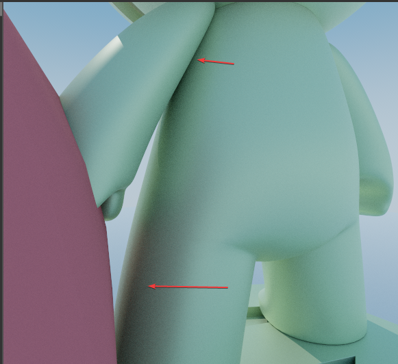
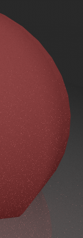
The Solution: Shadow Terminator Hacking

The shader implements Johannes Hanika's "shadow terminator hacking" technique to address these issues:

// Adjust shadow ray origin to match interpolated normals
float3 shadowPos = pointOffset(posObj, pos0, pos1, pos2, nrm0, nrm1, nrm2, barycentrics);
hit.shadowPos = float3(mul(float4(shadowPos, 1.0), objectToWorld4x3));

This technique adjusts the shadow ray origin so that shadows align more closely with the interpolated surface normals, reducing visual artifacts on low-poly geometry.

With	Without

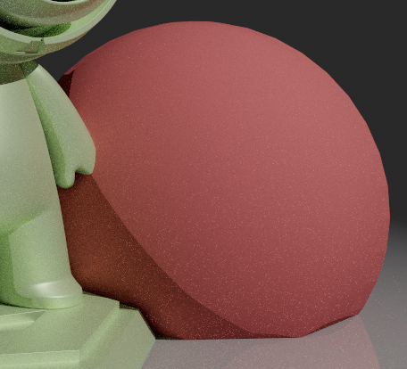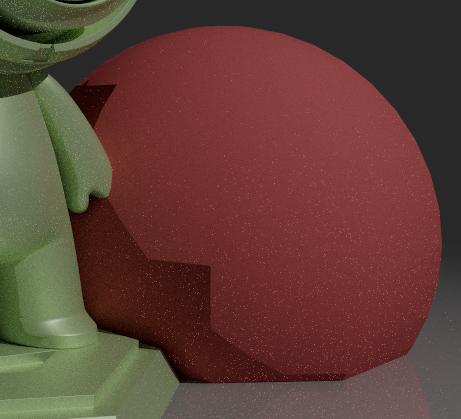Geometric vs Shading Normal Alignment

The shader implements sophisticated normal handling to prevent lighting artifacts:

// Calculate geometric normal from triangle edges (face normal)
float3 geonrmObj = normalize(cross(pos1 - pos0, pos2 - pos0));
hit.geonrm = normalize(mul(float4(geonrmObj, 0.0), objectToWorld4x3).xyz);

// Ensure geometric normal faces towards the ray origin (front-facing)
if(dot(hit.geonrm, worldRayDirection) > 0.0f)
    hit.geonrm = -hit.geonrm;

// Ensure shading normal and geometric normal are on the same side
if(dot(hit.geonrm, hit.nrm) < 0) {
    hit.nrm = -hit.nrm;  // Flip shading normal to match geometric normal
}

// For low-tessellated geometry, prevent internal reflection artifacts
float3 r = reflect(normalize(worldRayDirection), hit.nrm);
if(dot(r, hit.geonrm) < 0)
    hit.nrm = hit.geonrm;

With	Without

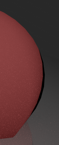Benefits of This Approach

• Addresses shadow terminator artifacts on low-poly models
• Reduces internal reflections on back-facing surfaces
• Helps maintain consistent lighting across triangle boundaries
• Can improve visual quality without requiring higher tessellation
• Compatible with existing assets without geometry modifications

Ray Query Characteristics

Performance Considerations

• Potential Reduced Overhead: May eliminate some shader binding table lookups and stage transitions (requires benchmarking for your specific use case)
• Cache Locality Trade-offs: Consolidating logic in one shader may improve cache locality for simple cases, but could increase instruction cache pressure for complex shaders
• Simplified Pipeline: Fewer pipeline state changes and shader stages

Development Characteristics

• Unified Control: All ray tracing logic in one place, which can simplify debugging for certain use cases
• Control Flow: Explicit procedural control within a single shader vs. pipeline stage transitions

Trade-offs: Ray Queries vs Traditional RT Pipelines

Both ray queries and traditional RT pipelines are capable approaches with different implementation characteristics:

Ray Queries May Be Preferred For:

• Integration into existing compute/fragment/mesh shaders for gradual adoption of ray tracing features
• Unified shader architectures where a single compute shader handles all material cases with explicit branching logic
• Algorithms requiring explicit procedural control within a single shader context
• Educational/research implementations where step-by-step ray control aids understanding
• Prototyping and experimentation where rapid iteration on ray processing logic is needed
• Simple to moderate complexity scenes where the unified approach doesn't create excessive shader complexity

Traditional RT Pipelines May Be Preferred For:

• Modular material systems where different materials benefit from specialized, optimized shaders
• Shader specialization with compile-time optimizations for specific material types
• Advanced ray tracing features like shader execution reordering (SER) and other hardware-specific optimizations
• Industry-standard workflows and established toolchain integration
• Complex scenes with many material types where shader modularity prevents excessive branching
• Memory-efficient payload handling with specialized payloads per ray type
• Large teams/codebases where shader modularity and separation of concerns is important
• Production renderers where driver optimizations and established patterns provide proven performance

Important Notes:

• Performance: Actual performance differences depend heavily on specific use cases, hardware, and implementation details
• Dynamic Materials: Ray queries use runtime branching in a single shader, while RT pipelines can use ubershaders or dynamic shader selection
• Complexity: The "best" choice often depends on your specific requirements, team expertise, and existing codebase

Technical Details

How to Trace a Ray with Ray Queries

1. Initialize the Ray Query

RayQuery<RAY_FLAG_NONE> q;  // Create ray query object
RayDesc ray = { origin, tMin, direction, tMax };  // Define ray
q.TraceRayInline(topLevelAS, RAY_FLAG_NONE, 0xFF, ray);  // Start tracing

2. Process Intersections

// For scenes with only opaque geometry:
while(q.Proceed()) {}  // Empty loop - opaque triangles auto-commit

// For scenes with mixed opaque/non-opaque geometry:
while(q.Proceed()) {
    if(q.CandidateType() == CANDIDATE_NON_OPAQUE_TRIANGLE) {
        // Force non-opaque triangles to be opaque (simplified alpha handling)
        q.CommitNonOpaqueTriangleHit();
    }
    // Note: CANDIDATE_TRIANGLE (opaque) is automatically committed
}

// After the loop completes, check the final committed status
if(q.CommittedStatus() == COMMITTED_TRIANGLE_HIT) {
    // Ray hit geometry - now we can extract intersection data
    float hitT = q.CommittedRayT();
    int instanceIndex = q.CommittedInstanceIndex();
    // Process the hit...
}

3. Extract Intersection Information

if(q.CommittedStatus() == COMMITTED_TRIANGLE_HIT) {
    // Get basic intersection data
    float hitT = q.CommittedRayT();
    int instanceIndex = q.CommittedInstanceIndex();

    // Get barycentric coordinates for interpolation
    float2 barycentrics = q.CommittedTriangleBarycentrics();

    // Get geometry data
    float3 worldPos = ray.origin + ray.direction * hitT;
    float3 normal = /* interpolate from vertex normals */;

    // Access material data using instance index
    MaterialData material = materials[instanceIndex];
}

Next Steps

• Denoising: Add temporal/spatial denoising to reduce sample count requirements
• Volumetrics: Extend to handle participating media and atmospheric effects
• Advanced Materials: Implement subsurface scattering or anisotropic BRDFs
• Performance: Benchmark ray queries vs traditional RT pipelines for your specific use case to determine the optimal approach

References

1. Hanika, Johannes. "Hacking the shadow terminator." Computer Graphics Forum, 2021. https://jo.dreggn.org/home/2021_terminator.pdf

2. Vulkan Ray Query Extension. "VK_KHR_ray_query." Khronos Vulkan Specification. https://registry.khronos.org/vulkan/specs/latest/man/html/VK_KHR_ray_query.html