Sample source
Browse the full sample on GitHub: raytrace_tutorial/19_ray_differentials
19 Ray Differentials - Tutorial
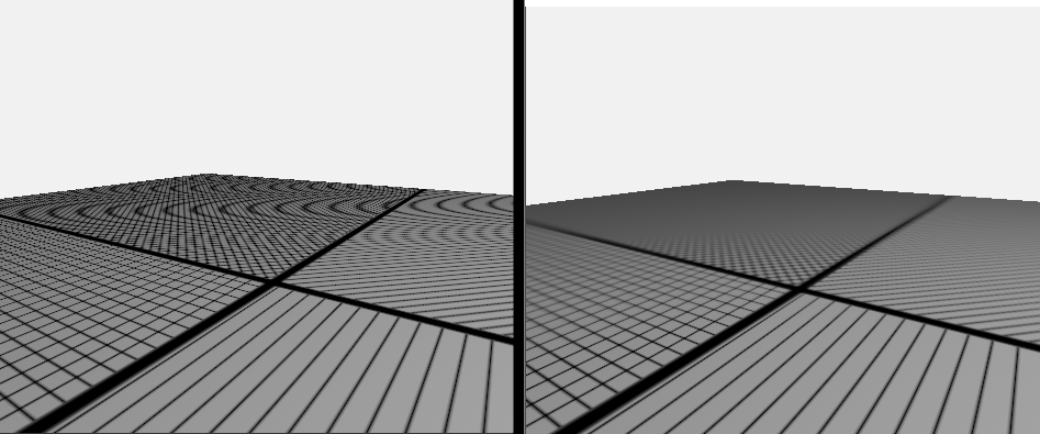
This tutorial shows how to drive texture filtering in a ray tracer using ray cones (Akenine-Möller et al., "Texture Level of Detail Strategies for Real-Time Ray Tracing", 2019). A rasterizer gets ddx/ddy for free from neighbouring fragments; a ray tracer does not, so without an explicit footprint every texture lookup samples mip 0 and high-frequency textures alias badly on slanted or distant surfaces. The screenshot above contrasts the un-filtered result (left) with the cone-driven trilinear result (right).
Key Takeaway: Two scalars per ray (width and spreadAngle) carried in the payload are enough to pick the right mip level on any triangle, including the surface-slant correction that an isotropic "screen pixel" approximation misses. Because the state lives in the payload, it propagates naturally to secondary rays.
Key Changes from 02_basic.cpp
1. Shader Changes - Ray cone carried in the payload
Modified: shaders/rtraydifferentials.slang
A ray's footprint at a hit is fully described by two scalars: the world-space diameter of the footprint at the ray origin (width), and the angular growth per unit travel (spreadAngle). Adding this two-float struct to the payload is the entire data-flow change required to support texture LOD on every ray in the pipeline.
struct RayCone
{
  float width;        // footprint diameter at the ray origin (world units)
  float spreadAngle;  // angular growth per unit travel (radians)
};

struct HitPayload
{
  float3  color;
  float   weight;
  int     depth;
  RayCone cone;       // <-- new
};
2. Shader Changes - Three helpers and the LOD computation
Modified: shaders/rtraydifferentials.slang
The LOD pipeline is three small functions, each doing one thing. The most important one is rayConeWorldFootprint — it is where the surface-slant correction lives:
// Cone diameter on the surface at the hit, with slant correction (1/|N.V|).
float rayConeWorldFootprint(RayCone cone, float hitT, float3 N, float3 V)
{
  float w = cone.width + cone.spreadAngle * hitT;
  return w / max(abs(dot(N, V)), 1e-3);
}
Two companion helpers in the same file complete the chain:
makePrimaryRayCone(projInv, viewportHeight)— initialise the cone for a pinhole camera.width = 0(camera is a point),spreadAngle = 2 * tan(fovY/2) / viewportHeight(the angular size of one screen pixel).triangleTexelDensity(wp, uv)— UV-per-world ratio on the hit triangle, computed assqrt(uvArea / worldArea).
In the closest hit, the LOD computation and the texture fetch are three lines. The third line is the propagation hook: a reflection/refraction ray spawned from this hit inherits the right footprint without any extra plumbing.
float worldFoot   = rayConeWorldFootprint(payload.cone, RayTCurrent(), N, V);
float uvFoot      = worldFoot * triangleTexelDensity(wp0, wp1, wp2, tex0, tex1, tex2) * pushConst.texGradScale;
payload.cone.width = worldFoot;    // propagate to the next bounce (if any)

albedo *= textures[material.baseColorTextureIndex]
            .SampleGrad(worldTexCoord, float2(uvFoot, 0), float2(0, uvFoot)).xyz;
3. Shader Changes - Primary ray initialisation
Modified: shaders/rtraydifferentials.slang (rgenMain)
The ray generation shader seeds the cone for the primary ray:
4. Data Structure Changes - Push constant for visualisation
Modified: shaders/shaderio.h
A single scalar multiplies the computed UV footprint so the user can scrub between under- and over-filtering at runtime:
struct TutoPushConstant
{
  // ... existing members ...
  float texGradScale = 1.0f;   // 0 = mip 0 (aliased), 1 = physically correct, >1 = blurred
};
5. C++ Application Changes - Mip chain on the texture
Modified: 19_ray_differentials.cpp (createScene)
The texture must be loaded with a full mip chain. nvsamples::loadAndCreateImage has a generateMipmaps flag that adds VK_IMAGE_USAGE_TRANSFER_SRC_BIT, sets mipLevels = nvvk::mipLevels(extent), and calls nvvk::cmdGenerateMipmaps after the staging upload — pass true:
nvvk::Image texture = nvsamples::loadAndCreateImage(
    cmd, m_stagingUploader, m_app->getDevice(), imageFilename,
    /*sRgb*/ true, /*generateMipmaps*/ true);
6. C++ Application Changes - Sampler must allow all mip levels
Modified: 19_ray_differentials.cpp (createScene)
A default-constructed VkSamplerCreateInfo has maxLod = 0, which clamps every fetch to mip 0 even when the gradient asks for a coarser mip. The sampler for a mip-chained texture must lift that clamp:
(All other fields are standard trilinear filtering with VK_SAMPLER_MIPMAP_MODE_LINEAR.)
7. UI Changes - Gradient scale slider
Modified: 19_ray_differentials.cpp (onUIRender)
0.0→ always mip 0 → strong moire.1.0→ physically correct LOD.>1.0→ over-blurred (useful to confirm coarser mips are actually reachable).
How It Works
The problem
For a screen-space pixel, the rasterizer hardware computes ddx/ddy of the interpolated UV across a 2x2 quad and feeds those gradients to the texture unit, which picks the right mip level (and direction for anisotropic filtering). Ray tracing has no such neighbourhood: each ray is independent. If you ignore this and call Sample(uv, 0), every fetch comes from mip 0 and any texture with detail finer than one screen pixel aliases.
The ray cone
Each ray is modelled as a thin cone. The cone has a starting diameter width at the ray origin and grows at an angular rate spreadAngle. At hit distance t, the cone diameter perpendicular to the ray is:
For a primary ray from a pinhole camera, width = 0 (the camera is a point) and spreadAngle = 2 * tan(fovY/2) / viewportHeight, which is the angular size of one screen pixel.
Surface slant
A perpendicular surface intercepts the cone as a disc of that diameter. A slanted surface intercepts it as a stretched ellipse — the major axis grows as 1/cos(theta), where theta is the angle between the surface normal and the view direction. For an isotropic approximation we use the worst case:
This single division is what kills the moire that the un-corrected pixelAngle * t formula leaves behind on grazing surfaces. The textured ground plane in this sample is the classic test case for it.
From world space to UV space
Once we have the world-space footprint diameter on the surface, we convert it to a UV-space length using the triangle's UV mapping density:
texelDensity = sqrt(|duv1 x duv2| / |we1 x we2|)    (UV units per world unit)

uvFootprint  = diameter_on_surface * texelDensity
That scalar is the isotropic gradient magnitude fed to SampleGrad(uv, (uvFootprint, 0), (0, uvFootprint)). The texture unit converts it to log2(uvFootprint * textureSize) and selects the matching mip with trilinear blending between adjacent levels.
Benefits
- Two scalars in the payload. No screen-space differentials, no neighbouring rays, no Gram-matrix inversion at the hit.
- Slant-correct. The
1/|N.V|term removes the aliasing that the naive pixel_angle x hitT form leaves on grazing surfaces. - Propagatable. Updating
cone.width = worldFootbefore a secondaryTraceRaycarries the right starting footprint to the next hit. The hit shader needs no special path for primary vs. secondary rays. - Stage-agnostic. The same helpers work for any closest-hit shader; the cone state is just data on the payload.
Technical Details
Why width exists even though it starts at 0
For the primary ray of a pinhole camera, width = 0 is correct — the ray emanates from a single point. The field becomes non-zero the moment a secondary ray is spawned from a hit: that ray's footprint at its origin is whatever the parent ray's footprint was at the hit (worldFoot). Without storing width, the propagation step couldn't preserve the accumulated coverage across bounces. This sample keeps width even though it never sets it to a non-zero value, so the abstraction is bounce-ready (see Going Further).
Isotropic vs. anisotropic filtering
SampleGrad here is given gradients of equal magnitude in U and V, so the texture unit performs isotropic trilinear filtering. The cost is some over-blurring along the long axis on extreme grazing surfaces, where true anisotropic filtering would preserve detail along the minor axis. For full anisotropy you'd need either:
- Ray differentials (Igehy 1999): carry
(dPdx, dPdy, dDdx, dDdy)per ray (12 floats) and compute proper anisotropic UV gradients at every hit, or - A two-cone variant of this technique that tracks
spreadAngleseparately in the screen X and Y directions.
For most use, the slant-corrected isotropic cone is the right point on the cost/quality curve.
Sampler and image usage flags
Two requirements on the Vulkan side often catch newcomers:
- Sampler:
maxLod = VK_LOD_CLAMP_NONE(or any value >= the number of mips). The default of0silently turns a mip-chained texture back into a mip-0-only texture. - Image usage: mip generation blits mip i into mip i+1, which requires both
VK_IMAGE_USAGE_TRANSFER_SRC_BITandVK_IMAGE_USAGE_TRANSFER_DST_BIT. TheloadAndCreateImagehelper addsTRANSFER_SRC_BITwhengenerateMipmaps = true;TRANSFER_DST_BITis added implicitly for staging.
Going Further: bounces and curved surfaces
This sample only traces primary + shadow rays, so the propagation hook is unused. Two small extensions take the technique to a full path tracer.
Inheriting the footprint at a bounce
06_reflection shows the iterative pattern (loop in rgenMain, no recursive TraceRay). To make reflections respect ray-cone LOD, the closest-hit shader writes the new cone state to the payload alongside the next ray:
payload.rayOrigin    = worldPos;
payload.rayDirection = reflect(-V, N);
payload.cone.width   = worldFoot;   // <-- inherit the hit-point footprint
// payload.cone.spreadAngle stays the same for a planar reflector
The next iteration's rchitMain then computes its own worldFoot from this inherited cone, gets the right mip on the reflected surface, and so on for every subsequent bounce.
Curvature augmentation for non-planar reflectors
A curved reflector causes the reflected cone to spread faster (concave) or slower (convex) than the incoming cone. Akenine-Möller et al. model this by adding a surface contribution to spreadAngle:
payload.cone.width        = worldFoot;
payload.cone.spreadAngle += 2.0 * surfaceSpreadAngle;   // beta, from per-triangle normal variation
surfaceSpreadAngle can be estimated from the variation of vertex normals across the triangle (section 20.6.2 of the paper). It is 0 for a flat triangle, so on plane.gltf the term contributes nothing — which is why this sample omits it. Add it as soon as a curved reflector enters the scene.
References
- Akenine-Möller, Crassin, Boksansky, Belcour, Meyer, Benty. Texture Level of Detail Strategies for Real-Time Ray Tracing. In Ray Tracing Gems, chapter 20 (NVIDIA, 2019) — the ray-cone formulation used here.
- Igehy. Tracing Ray Differentials. SIGGRAPH 1999 — the anisotropic alternative.